When creating software, one of the biggest challenges project managers face is figuring out the timeline, cost, and number of people required to complete the work. However, it is not always easy. That is where the Putnam resource allocation model comes in.
Lawrence H. Putnam developed this model in the late 1970s. It helps project managers make more intelligent decisions about time, effort, and resource allocation. It provides teams with a clearer picture of realistic goals when planning and executing software projects.
History of the Putnam Resource Allocation Model
Lawrence Putnam was the founder of the Putnam resource allocation model. He noticed that software projects followed predictable patterns just like in manufacturing and other engineering disciplines.
Putnam based this model on the Rayleigh manpower distribution curve, which had been used to model how effort builds up. From this, Putnam developed a formula that could estimate the effort required for a software project, based on its size and timeline.
This eventually became known as the Putnam resource allocation model, and it is the backbone of the well-known project estimation toolset called SLIM (Software Lifecycle Management).
Many organizations now treat the Putnam resource allocation model in software engineering as a first‑cut estimator, then refine numbers with story‑point velocity once Agile sprints begin.
What is the Putnam Resource Allocation Model?
The Putnam model can be described by the following equation.
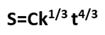
S = Size of the software (lines of code or function points)
Ck = Constant that reflects the team’s productivity (influenced by tools, skills, and processes)
E = Total effort (in person-months)
t = Time to complete the project (in months)
This equation shows that project size is related to effort and time. It is not a straightforward linear way, but rather a complex one. For example, if you try to cut the schedule in half, the required effort won’t be doubled; it would increase dramatically.
Let’s look at an example. Imagine you are planning a software product with the following parameters:
- 100,000 lines of code
- Based on previous projects, the Ck value of your team is 10.
If you plan for a 12-month schedule, the model can help you estimate the required effort in person-months. If you shorten the schedule to 6 months, the model will show that the required effort could triple. That means you would need a much larger team, which may not be realistic, and could even backfire due to increased communication overhead.
Benefits of using the Putnam Resource Allocation Model
- Realistic scheduling: Shows whether a proposed deadline matches the project’s size and the team’s historical productivity.
- Effort-vs-time trade-offs: Quantifies how much extra effort (person-months) a compressed schedule will cost.
- Workforce planning: Estimates the team size needed at each phase, helping managers avoid over- or under-staffing.
- “What-if” analysis: Predicts the impact of adding or losing developers partway through the project.
- Evidence for Brooks’s Law: Demonstrates that adding people to a late project can lengthen, not shorten, delivery time.
- Risk visibility: Highlights schedule or staffing plans that fall outside proven productivity ranges, allowing early course correction.
- Data-driven negotiation: Provides project leads with quantitative backing when pushing back on unrealistic timelines or headcount reductions.
Limitations of the Putnam Resource Allocation Model
Although the Putnam model predates modern DevOps, it still offers value when combined with today’s DORA metrics. The key is recognizing these limitations of the Putnam resource allocation model and adjusting inputs for iterative lifecycles.
- Size‑estimate sensitivity: If your LOC or function-point estimate is off, the entire effort and schedule prediction collapses.
- Calibration required: The productivity constant (Ck) must be derived from several past projects; without that history, results drift.
- Stable‑scope assumption: The model expects requirements to remain fixed. Frequent scope changes in Agile environments reduce its accuracy.
- Best for large, plan-driven projects: Overhead of data collection and calibration is hard to justify for small, fast-moving efforts.
- Ignores communication overhead: The formula does not explicitly account for the extra coordination time that large teams face.
- No cost-of-delay factor: It optimizes effort vs. time but does not weigh the business impact of shipping later vs. sooner.
Conclusion
The Putnam resource allocation model may seem somewhat outdated, but it remains highly effective. It proves that software development is not just about implementation; it is about planning properly and ensuring that the project goes smoothly.
This model analyzes size, time, and effort, providing a proper way to handle project feasibility, manage risks, and make allocations. If used properly, it can reduce the gap between planning and execution in software development.