The Difference Between Cognitive Complexity and Cyclomatic Complexity

Writing code is one thing. Understanding already written code is another.

Developers spend more time reading and understanding existing source codes than writing new ones. A simple script might be easy for you at first glance, but what happens when conditional statements, loops, and numerous dependencies are introduced? The more complex the code structure, the harder it is to modify, debug, and maintain.

Code complexity can be measured using two metrics: cyclomatic and cognitive metrics. One measures code by counting loops, branches, and decision points, while the other focuses on how difficult it is for developers to read and understand these pieces of code.

Let’s break down the differences and understand why both matter in your software development process.

Cyclomatic complexity is a software metric that measures how complex a program’s control flow is. Introduced by Thomas McCabe in 1976, it quantifies the number of independent paths in a codebase. In simple terms, it helps determine how difficult a program is to test, maintain, and debug by counting the different execution paths that can be taken.

For a better understanding, consider the number of different routes a car can take through a city. If it is on a simple road with no intersections, then it can only travel in one direction, making navigation easy. However, if the road has multiple turns, intersections, and traffic signals, the number of possible routes increases, making navigation more complex.

Cyclomatic complexity applies this concept to code, measuring the number of possible autonomous paths in a program.

Take a look at the Python script below:

Figure 1: A short Python script with low complexity

In the script above, there are four possible paths and three decision points (if, elif, and else), resulting in a cyclomatic complexity of four (one path for each condition and one for the default case).

• If the status is “pending,” it prints “Order is pending.”
• If the status is “shipped,” it prints “Order has been shipped.”
• If the status is “delivered,” it prints “Order has been delivered.”
• If none of these match, it prints “Invalid order status.”

Since there are only a few decision points, the cyclomatic complexity is low.

Now, compare it to the script below:

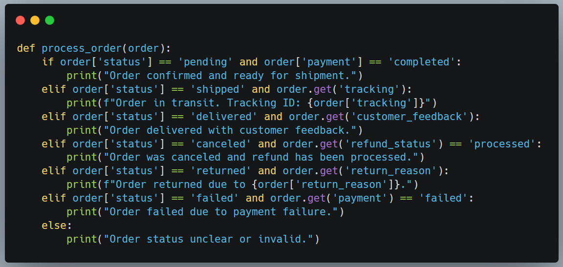
Figure 2: A Python script with higher complexity

In this script, there are seven possible paths, increasing the complexity:

• If the order is “pending” and the payment is completed, it prints “Order confirmed and ready for shipment.”
• If the order is “shipped” and tracking information is available, it prints “Order in transit. Tracking ID: [tracking]”
• If the order is “delivered” and customer feedback is present, it prints “Order delivered with customer feedback.”
• If the order is “canceled” and the refund has been processed, it prints “Order was canceled and refund has been processed.”
• If the order is “returned” and a return reason is given, it prints “Order returned due to [reason].”
• If the order is “failed” and the payment was unsuccessful, it prints “Order failed due to payment failure.”
• If none of these conditions match, it prints “Order status unclear or invalid.”

So, this script contains multiple conditions and nested checks, thereby increasing the number of possible paths.

Cyclomatic complexity is a comprehensive approach based purely on the number of independent paths in the code, but that doesn’t always mean a longer script is more complex or that a short script is always simple. A short script with deeply nested conditions, multiple logical operators in a single statement, or intricate loops can still have a high cyclomatic complexity.

For example:

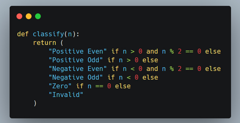
Figure 3: A shorter script with higher complexity

This function is short, but the complexity is higher because it has multiple logical conditions. Even though there aren’t many lines of code, the number of decision paths remains high, making it harder to read, test, and debug.

The script classifies a number as positive even, positive odd, negative even, negative odd, zero, or invalid using nested ternary operators. It first checks whether the number is positive or negative, then determines if it’s even or odd based on its value and divisibility by 2.

If the number is greater than 0, it checks whether it’s positive even (2, 4, 6) or positive odd (1, 3, 5). If it’s less than 0, it checks whether it’s negative even (-2, -4, -6) or negative odd (-1, -3, -5). If the number is zero, it returns “zero,” and any unexpected input defaults to “invalid.” This complexity comes from the multiple nested conditions, creating multiple execution paths.

Cyclomatic complexity itself isn’t just about length; it’s about the structure and how complex code is to test and maintain. Just because code has fewer paths doesn’t mean it’s easy to read.

How to measure cyclomatic complexity

Cyclomatic complexity is measured using the formula: M=E−N+2P

Where:

• M = Cyclomatic complexity
• E = Number of edges (connections) in the control flow graph
• N = Number of nodes (decision points and statements)
• P = Number of connected components (typically 1 for a single function)

Steps to measure cyclomatic complexity

1. Create a control flow graph: Write clearer codes and represent them as a flowchart where each control flow statement creates new branches.
2. Identify nodes and edges: Count the decision points (nodes) and the connections between them (edges).
3. Apply the formula: Plug the values into M = E – N + 2P to compute the complexity score.
4. Interpret the result: A higher value indicates more complex logic, making the code harder to test and maintain.

Cognitive complexity, first developed by James Bieri in 1955, is a software metric that measures how easy or difficult it is to understand and keep track of a piece of code, especially when the logic gets tangled or the flow takes unexpected turns.

Unlike cyclomatic complexity, which only counts the number of distinct paths, cognitive complexity attempts to quantify the mental effort or cognitive load required for code comprehension. It considers factors such as:

1. Nesting depth

Deep nesting of control structures (if statements, loops, etc.), as seen in example 2 above, significantly increases cognitive complexity level. Each level of nesting requires the developer to maintain additional context in their working memory.

2. Control flow breaks

Statements that interrupt the normal flow of code, such as break, continue, goto, or multiple return statements, add cognitive load because they force developers to track multiple exit points and state changes.

3. Logical complexity

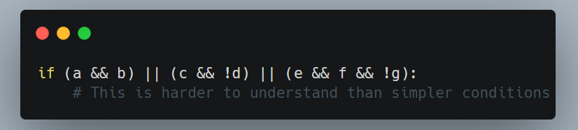
Complex boolean expressions, logical operators, and binary operators require more mental effort to understand. For example:

Practical benefits of low cognitive complexity

• Faster code reviews: Teams report faster and more regular code review cycles when working with code that has low cognitive complexity scores.
• Reduced technical debt: Low cognitive complexity makes code easier to read and modify.
• Better onboarding: New team members can understand and contribute to the codebase and write quality code, thereby increasing developer productivity.
• Code maintainability: Maintaining and reusing code blocks will be easier, and future modifications to different code sections will also be more straightforward.

Best practices for reducing cognitive complexity

To write cleaner, more understandable code:

• Use meaningful variable and function names: Self-explanatory names reduce the need for additional comments.
• Limit nesting levels: Too many indents make code difficult and more complicated to follow. Evaluate and check your current nesting level.

Avoid unreadable constructs and complex functions:

Take a look at the script below:

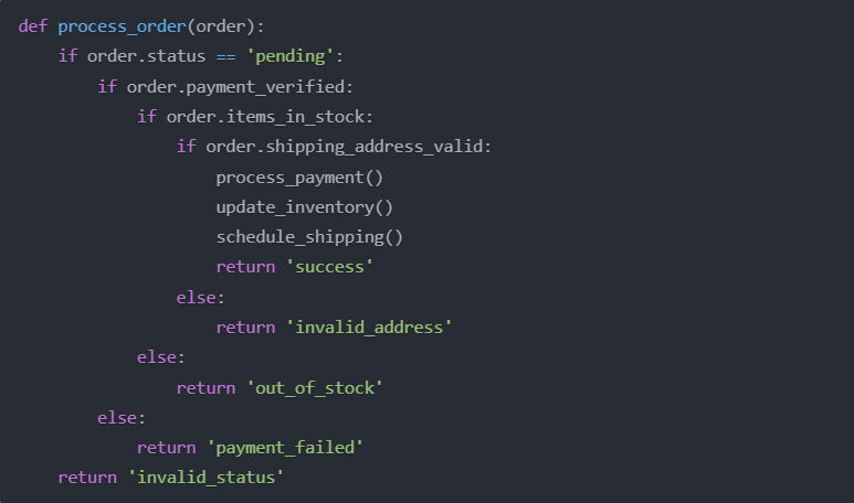
1. Then compare it with this:

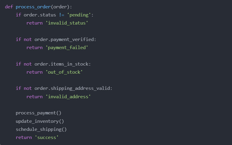
The second version has the same cyclomatic complexity as the first but lower cognitive complexity. It reads like a checklist rather than a nested maze.

• Finally, write self-documenting code: Your code should be intuitive enough that other senior software developers or even a junior developer can understand it without extensive explanations. Additional documentation for future references can come in if needed.

If your development teams ever struggled with a function that jumps between nested loops, conditionals, and callbacks, they’ve already felt the impact of high cognitive complexity.

Cyclomatic complexity and cognitive complexity both measure the complexity of code, but they focus on different aspects.

As mentioned earlier, cyclomatic complexity counts the number of execution paths in a program flow, helping developers test code coverage metrics. In contrast, cognitive complexity measures difficulty in terms of code readability, reusability, and maintainability.

Below is a comparison of their key differences:

Code complexity is a crucial aspect of software development. It’s not just about the number of choices that code makes; it’s also about how those choices are structured, how they fit together, and how easy it is for someone new to jump in and make sense of things. So, it’s not enough to write only functional code for computers. It is also important to write code that is easily readable by humans.

The real challenge isn’t choosing between cyclomatic and cognitive complexity but understanding how they complement each other. A good code should flow naturally and be easy to read at a glance without getting lost in excessive conditions.

As managing code complexity becomes increasingly crucial, industry trends suggest a move toward using AI-assisted refactoring tools like MilestoneAI to suggest code clarity and coding standards and provide real-time feedback. Click here to see a demo.